Extreme and Highly Heterogeneous Microclimates in Selectively Logged Tropical Forests

Introduction

Tropical forests host the majority of terrestrial species diversity, and generate the majority of terrestrial nutrient and water fluxes (Malhi et al., 1999). They also are being increasingly affected by fire, clearance, selective logging, and urbanization (Chazdon, 2003; Newbold et al., 2015) which all contribute to a highly heterogeneous mosaic of disturbed patches. Understanding microclimate variation in these systems will be critical for predicting how the organisms that comprise them will respond to large-scale global change, e.g., for recruitment dynamics of tree seedlings (Brokaw, 1985), for behavior of ground-dwelling animals (Vitt et al., 1998), or for spatial dynamics of soil respiration (Raich and Tufekciogul, 2000). Specifically, knowledge of microclimate can improve estimates of species richness (Stein et al., 2014), functional diversity (Bergholz et al., 2017; Stark et al., 2017), demography (Baraloto and Couteron, 2010; Uriarte et al., 2018), and carbon fluxes (Raich and Schlesinger, 1992). Microclimate is also especially important in predicting species' responses to climate change because the existence of microrefugia provide conditions suitable for persistence without requiring rapid dispersal (Klein et al., 2009; Meineri and Hylander, 2017).

Disturbances can affect tropical forests' ability to buffer changes in their microclimate from changes in broader-scale climate (Ewers and Banks-Leite, 2013; De Frenne and Verheyen, 2016). For example, selective logging may cause reductions in canopy closure that in turn drive increased radiation and airflow, which then lead to decreased broad-scale climate buffering and higher variation in microclimate (Fauset et al., 2017). The extent of these effects remains controversial (Senior et al., 2017b). On the one hand, a recent study has suggested that selective logging in Borneo leads to very small changes in thermal microclimate (Senior et al., 2017a). On the other hand, a different Bornean study of selective logging and forest conversion to oil palm show that disturbance increases mean air temperatures and reduce relative humidity and soil moisture (Hardwick et al., 2015). Other studies have shown that fire (Didham and Lawton, 1999) and logging (Fetcher et al., 1985; Senior et al., 2017b) have similar effects on reducing buffering of forest microclimate from broad-scale climate variation.

Regardless, variation in microclimate within forests remains poorly empirically quantified relative to variation in broad-scale climate across forests [but see (Scheffers et al., 2017; Senior et al., 2017b)]. The effects of anthropogenic disturbance (Foley et al., 2005) may occur primarily at much smaller spatial and temporal scales (Bellard et al., 2012). There is a need to better predict how large-scale climate variation translates to small-scale microclimate variation (De Frenne and Verheyen, 2016). Microclimates have been difficult to predict at small temporal and spatial scales. Most weather station data come from open rather than forested areas. Weather stations placed in open clearings are limited in their utility for predicting microclimate within forests or other complex environments.

Additionally, the microclimate experienced by organisms or patches within forests may differ strongly from the air temperatures measured by nearby weather stations. The temperature of an object is determined not only by air temperature, but also by other heat fluxes comprising the energy balance. These fluxes include radiation (from shortwave sources, e.g., sunlight, and longwave sources, e.g., blackbody radiation dependent on the emissivity and albedo of the object), convection (including evaporation), and conduction. Air temperature can play a role in all of these fluxes but may not always be the primary factor driving temperature. Predicting how air temperature transfers to organismal temperature remains challenging, but important for understanding how disturbance affects organismal performance across space and time.

To address recent calls to better measure within-forest microclimate (De Frenne and Verheyen, 2016), and to better assess the impact of disturbance, we posed three questions:

1) Does selective logging drive increased heterogeneity and extremes in forest microclimate, and if so by how much?

2) To what extent can on-plot or off-plot weather station data be used to predict forest microclimate?

3) Can forest structure and topography predict forest microclimate across time and space?

We focused our empirical measurements in Sabah, Borneo Severely degraded forests (with multiple recent road construction events) represent 32% of logged forest area in Sabah (Bryan et al., 2013), with some logging affecting over 70% (Potapov et al., 2017). In contrast to previous studies that measured air temperature, we measured a microclimate thermal proxy sensitive to radiative, convective, and conductive heat fluxes. This thermal proxy is relevant to a range of organismal processes including plant regeneration, animal behavior, and soil nutrient fluxes. Measurements were made across space and time within three 1-ha plots comprising a gradient from old growth to heavy selective logging. We then combined these data with nearby weather station air temperature data, as well as measurements of topography and canopy structure derived from detailed ground surveys and airborne LIDAR.

Materials and Methods

Study Location

We identified three sites along a logging intensity gradient in the Malaysian state of Sabah in Borneo. Sites each contain a 1-ha plot in lowland mixed dipterocarp forest, and are part of a long-term investigation into the effects of forest fragmentation (Ewers et al., 2011). These sites are managed by the Global Ecosystem Monitoring network and are given standardized names in the ForestPlots database (https://www.forestplots.net).

The plots are chosen to contrast an unlogged old growth forest with a moderately logged forest and a heavily logged forest (Riutta et al., 2018). Locations and details are given in Table 1. The first plot, MLA-01, is representative of old-growth forest conditions, and is referred to as “old growth” (Figure 1C). The plot is located within the Maliau Basin Conservation Area, is characterized by topography with several hills and a stream drainage and contains mature forest with an open understory. The logged plots are located within the Stability of Altered Forest Ecosystems (SAFE) Project (Ewers et al., 2011) in Kalabakan Forest Reserve. The area has been selectively logged for the first time in the mid 1970s, followed by one to three rounds of logging between 1990 and 2008. The cumulative extracted biomass in the area ranged from 46 to 54 Mg C ha⁻¹, and the total biomass loss, including collateral damage, increased post-logging mortality and abandonment of some of the felled stems was estimated to be 94–128 Mg C ha⁻¹ (Struebig et al., 2013; Pfeifer et al., 2016; Riutta et al., 2018). Mean extraction volumes are estimated to be 150–179 m³ ha⁻¹, compared to 152 m³ ha⁻¹ across all of Sabah (Fisher et al., 2011). The SAF-03 plot (within SAFE Project Fragment E), is representative of moderate selective logging (current biomass equals 47% of pre-logging biomass) and is referred to as “moderately logged” (Figure 1B). The plot is characterized by a sloped topography and contains a mature forest with several gaps caused by logging of large trees. The SAF-01 plot (within SAFE Project Fragment B), is representative of heavy selective logging (current biomass equals 14% of pre-logging biomass), and is referred to as “heavily logged” (Figure 1A). The plot is characterized by an undulating topography and a stream, with some mature trees and several large logging gaps.

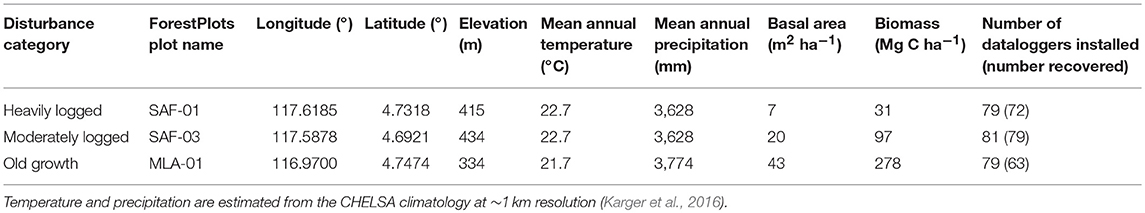
Table 1. Summary information for each plot including datalogger deployment statistics.

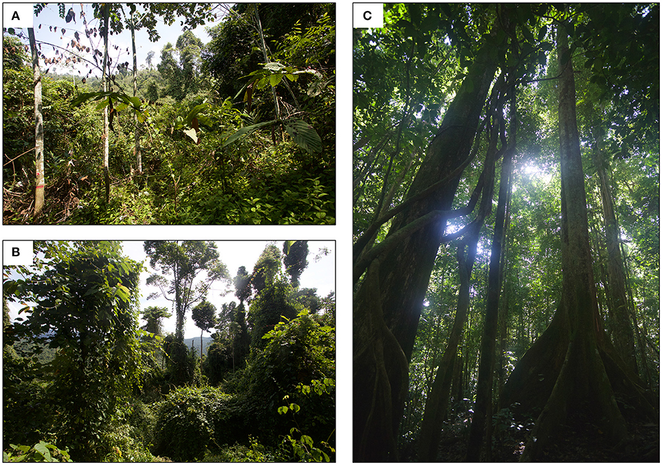
Figure 1. Representative conditions within (A) the heavily logged plot, (B) the moderately logged plot, and (C) the old growth plot.

Microclimate

To map the microclimate thermal proxy in each plot, we installed dataloggers on a semi-regular grid pattern varying in minimum distance from 1 to 14 meters. Each datalogger was a Thermochron iButton (DS1921G, Maxim), capable of logging up to 2048 temperature values between −30 and 70°C. Each datalogger was waterproofed by wrapping in plastic paraffin film (Parafilm, Bemis) and then in light yellow duct tape (Figure S1). Dataloggers were attached using plastic zip-ties onto PVC stakes at a height of 1–3 cm immediately above the forest floor. The tape color was chosen to approximate the albedo of vegetation/soil, and the size of the sensor package was chosen to have a similar boundary layer to many small organisms (e.g., tree seedlings, fallen branches, large insects). The sensor packages intentionally did not include a radiation shield, as the intent was not to measure air temperature. Temperatures recorded by the loggers therefore reflect a combination of conductive, convective, and radiative heat fluxes, and can be considered a rough proxy for those experienced by small organisms.

Each plot contains 25 20 × 20 m² subplots, demarcated by 1 m-high PVC stakes embedded in the soil. Each subplot also contains at its center a mesh litter trap suspended on PVC stakes at 1-m height. Exact locations for all subplot corner and center stakes were determined using ground-based Field-Map software [IFER, Jílové u Prahy, Czech Republic (Hédl et al., 2009)]. Spatial positions were recorded in three-dimensional space (local x, y, z-coordinates) using an Impulse 200 Standard laser rangefinder and MapStar Module II electronic compass (Laser Technology, Colorado, USA).

We installed a datalogger on these stakes at the corner of each subplot and the center of each subplot. We also chose at random three focal subplots in each plot for higher-resolution sampling. Within these subplots we established a cross-type design, with six additional dataloggers deployed at 1–5 m distance on additional PVC stakes located near each litter trap (Figure S2). A total of 239 dataloggers were installed.

Dataloggers were deployed during the end of the dry season in late 2015. Each recorded 28 days of data at 20-min intervals (Data Sheet S1). Start times were synchronized among dataloggers within plots. The exact date of deployment was 1 November for the heavily logged plot and 9 November for the moderately logged and old growth plot. Weather conditions during November–December 2015 were consistently dry and hot, so we do not anticipate any biases from the differing start dates. In nearly all cases dataloggers were recovered in their original location, except for a small number that were transported 1–2 meters down slopes. We treated data from these as though they were in their original position. A small number of dataloggers also failed due to being lost or punctured by animal bites. 90% of dataloggers (214/239) were successfully recovered and downloaded (Table S1). Missing data was random across space and plots (Figure S3).

Air Temperature Data

To compare the microclimate thermal proxy to other temperature metrics, we obtained off-plot (open site) and on-plot (below canopy) weather station data (Data Sheet S3). To represent off-plot data for both the moderately and heavily logged plots, a weather station was located in a cleared area at the SAFE base camp (4.724341°N, 117.601449°E), at a distance of 2.0 km from the heavily logged plot and 3.9 km from the moderately logged plot. Data were logged continuously (Datahog, Skye Instruments, UK). Measurements included air temperature (°C) and photosynthetically active radiation (W m⁻²). Data were available for all of the study period. To represent off-plot data for the old growth plot, another weather station was located in a cleared area at the Maliau Basin Studies Center (4.736263°N, 116.97662°E), at a distance of 1.4 km from the plot. Available data only included photosynthetically active radiation (W m⁻²). Data were available for ~25% of the study period. We predicted air temperature values at this plot for these dates by calibrating a LOESS regression model of air temperature based on time of day (seconds after midnight) and photosynthetically active radiation, calibrated with weather station data from an open clearing at the SAFE base camp (78 km distance, 184 m lower elevation). Because of the small elevation change we did not include a further lapse rate correction for temperature. The fitted model, which had a residual standard error of 0.9°C, was used to predict off-plot air temperature at the old growth plot (Figure S4).

To represent on-plot air temperature, we located air temperature sensors (HOBO, U23-002) within radiation shields at 1.5 m height in a subplot within each plot (corresponding to a focal subplot with a higher density of microclimate dataloggers: old growth, subplot 18; moderately logged, subplot 24; heavily logged, subplot 25). Temperature was measured hourly. Locations of subplots are indicated in Figure S3.

LiDAR Data

Discrete airborne LiDAR data were acquired by NERC's Airborne Research Facility (ARF) in November of 2014 using a Leica ALS50-II LiDAR sensor flown on a Dornier 228-20 at 41 points m⁻² density, with up to four returns recorded per pulse. Georeferencing of the point cloud was ensured by incorporating data from a Leica base station in the study area. LiDAR point clouds were classified into ground and non-ground points, and used to produce a 1 m resolution canopy height model by averaging the first returns (Data Sheet S2). Gaps in the canopy height model were filled by averaging neighboring cells.

Topography

The ground-mapped coordinates of the subplot corners, subplot centers, and all stems were used to construct a digital elevation model (DEM) for the plot. Elevation was interpolated onto a 1 m grid using ordinary kriging with a minimum of 4 points and search radius of 30 meters. This grid was then aligned to the LIDAR-determined location and elevation of the plot corners. The DEM was then used to estimate slope (in degrees) and cosine of aspect (with higher values indicating more southerly exposures) for each location (Data Sheet S2).

Forest Structure

Forest structure was determined from field surveys and from airborne laser scanning (Data Sheet S2). For the field survey, all trees ≥10 cm diameter at 1.3 m height were censused in each plot in 2016. The census followed the RAINFOR protocol (Phillips et al., 2016). Diameter was measured at 1.3 m with a tape measure, height with laser rangefinders, and x-y position of each stem were determined using the same system as the subplot corners. The horizontal crown projection of every tree was mapped by measuring spatial positions (x and y-coordinates) of 5–30 points (depending on the size of the crown) at the boundary of a crown projected to the horizontal plane and then smoothed using Field-Map software.

Field stem maps were then converted into raster grids of stem basal area density (smoothed with 2-m Gaussian kernel, and then rasterized to 1 m resolution), canopy density (number of overlying canopies per unit area; 1 m resolution), and plant area index (PAI) (10 m native resolution, interpolated to 1 m resolution). Spatial variation in PAI was mapped from the LiDAR point cloud using the MacArthur-Horn method (MacArthur and Horn, 1969). The method assumes that the leaves are randomly distributed within the laterally homogeneous canopy layers, so the PAI is proportional to the logarithm of the fraction of LiDAR pulses, β, penetrating through the canopy: $\text{PAI}=-\frac{1}{\kappa }ln(\beta )$, where κ is a correction factor that accounts for canopy features, such as clumping and the distribution of leaf angles. We assumed a constant value of κ = 0.7, which is within the range reported by Stark et al. (2012). Only the first returns, representing the first interaction of each LiDAR pulse with the canopy, are considered. We employed a lower cutoff of 2 m to avoid confusing ground returns with low-lying vegetation. PAI was estimated for point locations along a 1 m regular grid using circular sampling neighborhood of 10 m. This sampling window size is used to capture a sufficient number of LiDAR returns to avoid saturation effects in the more densely vegetated parts of the plots. This approach for calculating canopy closure may be biased, as clumping of vegetation, variation in leaf angle, and canopy edges (i.e., at gaps) should lead to spatial variation in the κ coefficient. It was not possible with our data to constrain κ using hemispherical photos due to saturation effects. While clumping can be estimated from terrestrial LiDAR data (Jupp et al., 2009), the high pulse densities required preclude this approach from being used with airborne LiDAR data. Other approaches for using airborne data to estimate clumping in airborne LiDAR data have led to significant negative biases in PAI estimates in our trial analyses (Detto et al., 2015). We therefore acknowledge that the constant-clumping approach may introduce some unknown spatial biases into our PAI estimates, but believe that the chosen approach is reasonable given currently available methods.

Statistical Analysis

To summarize variation in microclimate data across time, we computed spatial minima, means, maxima, and ranges at each time, combining information across all dataloggers. Variograms across all dataloggers within each plot also were estimated to assess spatial autocorrelation at each time. We also summarized the commonality of extreme heat events at each datalogger by calculating a time series of the presence of temperature spikes above 35°C that persisted for at least 20 min. Point estimates are reported with standard deviations.

To summarize variation across space, we computed temporal minima, means, maxima, and ranges at each datalogger, combining information across all times. To compare the similarity of time series of microclimate data to the weather station air temperatures, we merged datasets at the frequency of the weather station data. Microclimate time series included spatial minimum, mean, and maximum values of the microclimate thermal proxy at each time point. We then calculated the Pearson correlation and absolute deviations between each microclimate and off-plot/on-plot weather station air temperature time series. For visualization purposes (Figure 5; Movies S1–S3) we also spatially interpolated the spatial microclimate datasets using cubic splines to 1 m resolution. These interpolations were not used in quantitative analyses.

To determine which factors predicted variation in microclimate over space, we obtained minimum, mean, and maximum values of the microclimate thermal proxy at each location (n = 214). We then extracted values of a set of spatial predictors at each location as the mean value in a 10 m buffer region. Predictors comprised elevation (after subtracting plot mean values for each plot to provide a relative index of height), slope, cosine aspect, basal area density, canopy height, canopy density, plant area index, and biomass fraction removed (calculated at plot level). Pearson correlation coefficients between any pair of predictor variables took a mean value of 0.38 and never exceeded 0.78 (for canopy height and PAI). Subsequently we fit linear mixed models using each of minimum, mean, or maximum microclimate thermal proxy values as the dependent variable. Each model included the spatial predictors as fixed effects, plus a random intercept for plot, and a Gaussian spatial correlation structure, with parameters fit from the data. All predictors were scaled (z-transformed) before analysis to enable interpretation of fixed effect estimates as effect sizes. The model therefore treats the plots as independent samples along a selective logging gradient, while simultaneously accounting for the hierarchical structure of the data (some variables measured between plots, others within), and for spatial autocorrelation among data loggers. Explained variation for fixed and fixed plus random effects for each model was summarized using Nakagawa's pseudo-R² statistic (Nakagawa and Schielzeth, 2013).

All statistical analyses were conducted in R version 3.3.3. Summary statistic distributions are reported as mean ± standard deviation. Spline smoothing was carried out with the akima package; GIS analyses with the rgdal, sp, maptools, and raster packages; LiDAR data processing with the lidR package; linear mixed models with the nlme and MuMIn packages.

Results

We obtained a total of 444,416 temperature measurements at 214 locations representing a total of 30,000 m² of forest, with 63–79 loggers successfully recording data within each plot (Table 1). Animations of the spatio-temporal variation of the microclimate within each plot over the study period are provided as supporting files Movies S1–S3.

Question 1: Does selective logging drive increased heterogeneity and extremes in forest microclimate, and if so by how much?

Spatial microclimate patterns at the forest floor, calculated by averaging all time points, differed between plots and were consistent with more variation and higher extremes in more heavily logged plots (Figure 2). The distribution of mean microclimate thermal proxy values was lowest in the heavily logged and higher in the moderately logged and old growth plots. Mean minimum microclimate thermal proxy values were statistically different (but small; <1°C) between moderately logged and old growth plots (21.5 vs. 21.3°C; t-test p < 10⁻³, df = 140) and between old growth and heavily logged plots (20.5 vs. 21.3°C; t-test p < 10⁻¹⁵, df = 132). Mean maximum microclimate thermal proxy values at each location were statistically different in both moderately logged (32.8 vs. 28.6°C; t-test p < 10⁻¹⁵, df = 122) and heavily logged (31.6 vs. 28.6°C; t-test p < 10⁻³, df = 118) plots relative to old growth. Some locations in both logged plots experienced much higher maxima (50°C in moderately logged and 52°C in heavily logged vs. 44°C in old growth). Consistent with this finding, microclimate thermal proxy ranges were statistically different in moderately logged (11.3 vs. 7.3°C; t-test p < 10⁻⁵, df = 124) and heavily logged (11.1 vs. 7.3°C; t-test p < 10⁻⁵, df = 118) plots relative to old growth.

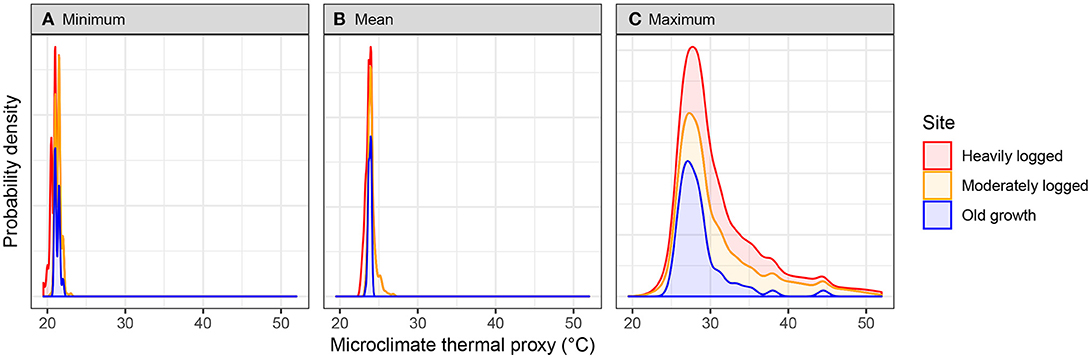
Figure 2. Spatial distributions of microclimate thermal proxy values at each plot over the 1-month study period for (A) minimum, (B) mean, and (C) maximum values. Note y-axis scale varies between panels.

Temporal microclimate patterns, calculated by averaging data from all dataloggers within a plot, were also consistent with more variation and higher extremes in the logged plots (Figure 3A). Over diurnal cycles, spatial minimum and mean temperature peaks occurred at ~11 a.m., with all temperature excursions constrained between 20 and 30°C. However, differing patterns occurred for maximum temperatures over diurnal cycles: in both logged plots, maximum temperatures reached upper values close to 10 a.m. (typically the brightest part of the day before clouds set in), with many temperature excursions exceeding 45°C, while in the old growth plot the upper value was obtained closer to 11 a.m., with values never exceeding 45°C.

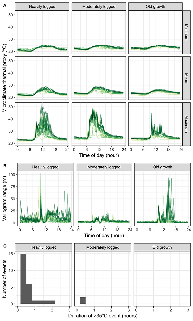
Figure 3. Temporal patterns in microclimate thermal proxy values. (A) Diurnal traces of minimum, mean, and maximum temperature (across dataloggers) for each plot. (B) Diurnal traces of variogram range (higher values indicate higher spatial heterogeneity), for each plot. Traces are colored by day, with earlier dates in orange and later dates in purple. (C) Frequency of extreme thermal events where microclimate thermal proxy values exceeded 35°C for a duration of time.

Heterogeneity in microclimate thermal proxy values also varied temporally across plots (Figure 3B). The semivariogram range (the distance at which spatial correlation between samples first flattens, providing a metric of spatial heterogeneity) in each plot changed over the course of the day at each plot. The lowest values occurred at nighttime in all plots, consistent with uniform plot cooling. Daytime patterns varied strongly between plots. Across all times, the moderately logged plot was not statistically different from the old growth plot (3.5 vs. 3.6 m, t-test p = 0.6, df = 2484). However, the heavily logged plot was statistically different from the old growth plot (7.3 vs. 3.6 m, t-test p < 10⁻¹⁵, df = 4036). Additionally, these time-series all had distinct peaks at certain times of day that were consistent across days, indicating consistent localized heating patterns. The peaks in heterogeneity occurred primarily in the morning in the heavily logged plot, and in the mid-afternoon in the old growth plot.

Logged plots experienced more and longer extreme thermal events than the old growth plot (Figure 3C). The heavily logged plot experienced more than 20 events in which a datalogger recorded a temperature exceeding 35°C for more than 20 min, and several events lasting more than an hour. The old growth plot never experienced any such events.

Question 2: To what extent can on-plot or off-plot weather station data be used to predict forest microclimate?

Off-plot air temperature time series poorly predicted microclimate thermal proxy time series (Figures 4A,C). Mean minimum microclimate thermal proxy values were biased at all plots, with off-plot weather stations estimating values that were 2 ± 4°C higher than recorded by the dataloggers (Pearson's ρ, 0.70–0.88). Average mean microclimate thermal proxy temperatures were also biased across all plots, with off-plot weather station values 1 ± 4°C higher than recorded by the dataloggers (Pearson's ρ, 0.75–0.93). Mean maximum microclimate thermal proxy values were biased in the old growth plot by 1 ± 5°C (Pearson's ρ, 0.65) and were more strongly biased in the two logged plots, with off-plot weather station values 4–7 ± 8°C lower than recorded by dataloggers (Pearson's ρ, 0.30–0.75).

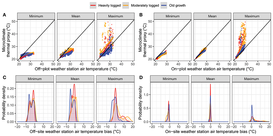
Figure 4. Coordination between microclimate thermal proxy values and air temperature measured either (A,C) by off-plot weather station in open clearing or (B,D) on-plot weather station. (A,B) indicate correlations between air temperature and each of minimum, mean, or maximum microclimate thermal proxy values (across dataloggers) at each time. The 1:1 line is shown in black. (C,D) indicate the distributions of deviations between microclimate thermal proxy values and air temperature.

On-plot air weather station air temperature data better predicted microclimate thermal proxy values (Figures 4B,D). Across plots, mean minimum on-plot air temperature values were biased by 1 ± 1–2°C higher than observed by dataloggers (Pearson's ρ, 0.87–0.94). Mean on-plot air temperature values were unbiased across plots (0 ± 1°C; Pearson's ρ, 0.94–0.98) while maximum on-plot air temperature values were biased lower than those recorded by dataloggers in the old growth by 2 ± 3°C (Pearson's ρ, 0.64), by 6 ± 7°C in the moderately logged plot (Pearson's ρ, 0.58), and by 4 ± 4°C (Pearson's ρ, 0.79) in the heavily logged plot.

Question 3: Can forest structure and topography predict forest microclimate across time and space?

Forest structure was highly variable across and within the three plots, with maximum canopy height varying from 0 to 77 m, basal area density from 0 to 0.04 m² m⁻², canopy density from 0 to 6 tree crowns m⁻², and PAI from 0 to 13 m² m⁻². Similarly, plot topography was also variable, with elevation from 324 to 475 m, with both north and south aspects, and with slope variation from 0 to 58°. Details of ranges within each disturbance type are visualized in Figure 5 and summarized in Table 2.

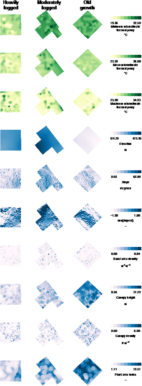
Figure 5. Spatial patterns of microclimate thermal proxy values, topography, and forest structure. For each plot, data for minimum, mean, and maximum microclimate thermal proxy values are shown, as well as site elevation, plot slope, cosine aspect, basal area density, canopy height, canopy density, and plant area index. Color scales are consistent within each variable (column). Each pixel represents 1 m. Ranges are given in Table 2.

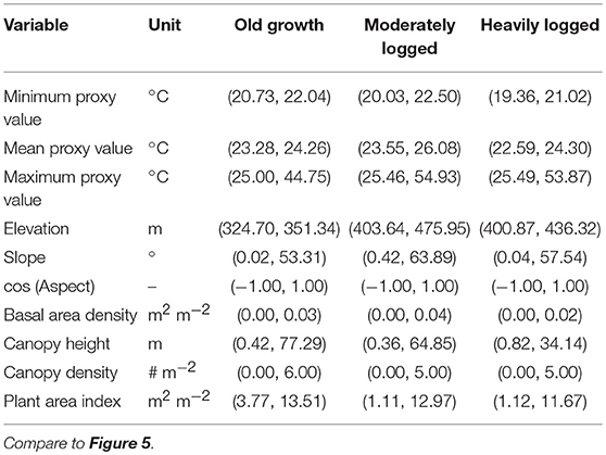
Table 2. Ranges of variation in microclimate thermal proxy values and key topographic and forest structure variables.

Both forest structure and topography contributed to spatial distributions of the microclimate thermal proxy, though the effects of each predictor depended on the type of temperature (Figure 6). Most standardized coefficient estimates in each model were small (absolute magnitudes of <0.1 sd sd⁻¹), though there were several notable exceptions (Figure 7A). For the model of minimum microclimate thermal proxy values, there was a negative effect of biomass removal (−0.1). For the model of mean microclimate thermal proxy values, there was a positive effect of canopy height (+0.3) and a negative effect of plant area index (−0.2). For the model of maximum microclimate thermal proxy values, effects were much stronger. There was a positive effect of relative elevation (+0.2), canopy height (+3.1), tree density (0.3), and biomass removal (+2.6), as well as a negative effect of slope (−0.6), cosine aspect (−0.5), basal area (−0.1), and PAI (−2.7).

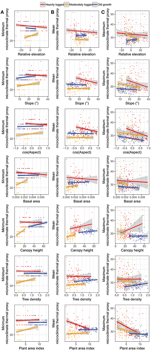
Figure 6. Pairwise relationships between plot topography and forest structure and (A) minimum microclimate thermal proxy values, (B) mean values, and (C) maximum values. Points represent locations of individual data loggers, colored by plot.

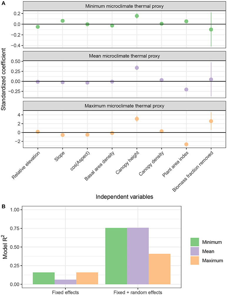
Figure 7. Summary of regression models of microclimate thermal proxy values. (A) Standardized estimates of fixed effects (points) and 50% confidence intervals (vertical lines) in each model. Note different y-axis scales on each facet. (B) R² values for models of minimum, mean, and maximum microclimate thermal proxy values.

Fixed effects explained 16% of minimum values, 6% of mean values, and 16% of maximum values of the microclimate thermal proxy (Figure 7B). Fixed effects and the site random effect together explained between 40 and 76% of the variance, suggesting that unmeasured factors were also important drivers of microclimate thermal proxy values.

Discussion

We found that selectively logged forests experienced more heterogeneous, hotter, and consistently extreme microclimate thermal proxy values than old growth forest. We found consistent differences of >10°C occurring at 1–5 meter spatial scales. These ranges of variation are consistent with prior studies of air temperature heterogeneity within forests (Scheffers et al., 2017) and have broad implications for climate change responses: the environments experienced by organisms may potentially expose individuals (especially for sessile organisms) to extreme conditions not predicted in fine-scale air temperature data or in broader-scale climate data (Baraloto and Couteron, 2010; Scherrer and Körner, 2010; Stark et al., 2017). Unlike in alpine systems where environmental heterogeneity provides thermal refugia that buffer climate change (Scherrer and Körner, 2010), heterogeneity in this warm forest is likely to exacerbate it. Our findings at fine spatial scales and biologically relevant temperatures thus build on other studies that have argued for disturbance driving strong warming and less buffering of climate change (De Frenne et al., 2013; Hardwick et al., 2015; Senior et al., 2017b).

The temperatures characterized by our microclimate thermal proxy were more heterogeneous and extreme than the air temperatures measured by weather stations. This finding is in line with another study of within-forest surface temperature heterogeneity that used thermal imaging methods (Scheffers et al., 2017). This outcome challenges the possibility of downscaling weather data from stations in open clearings to predict climate impacts at fine scale within forests. Our study echoes recent calls to better measure thermal environments at scales and locations that are relevant to the organisms of interest (Körner and Hiltbrunner, 2017), and provides one of very few high resolution records of such variation (Scheffers et al., 2017; Senior et al., 2017a).

We found that forest structure was a stronger driver of maximum microclimate thermal proxy values than of minimum or mean values. Maximum microclimate thermal proxy values increased with several variables but primarily increased with taller canopies (i.e., with more variation allowing oblique light transfer), lower plant area index, and higher biomass fraction removed. Mean microclimate thermal proxy values showed similar trends and increased with canopy height and decreased with higher plant area index. In contrast, minimum microclimate thermal proxy values increased with higher canopies and lower biomass fraction removed but was largely similar within and across plots. This latter finding is consistent with uniform night-time cooling of air masses, with limited variation in wind or sky exposure (i.e., convective and radiative heat fluxes), as primarily determined by regional processes. In all cases, other unmeasured site-level factors (reflected by random effects variances) not related to forest structure, biomass removal, or topography explained large fractions of the remaining variation. Our results therefore suggest that fine-scale variation in thermal environment remains difficult to predict even with detailed knowledge of forest structure and topography.

The drivers of maximum and mean values of the microclimate thermal proxy are consistent with selective logging primarily affecting canopy structure, leading to to higher radiation loading and ultimately driving more extreme and heterogeneous maximum temperatures (Chazdon and Pearcy, 1991). Diurnal cycles of temperature change indicated that specific locations were consistently warmer than others, and that these peaks in temperature also occurred at consistent times of day. While the canopy height and PAI data capture the broad distribution of logging-caused light gaps, it was not possible to use the airborne LiDAR data to propagate light transfer through the lower canopy due to lack of data for understory vegetation structure [but see (Webster et al., 2017)]. The understory vegetation likely determines the conditions experienced at the forest surface, and thus determines the spatial variation in microclimate thermal proxy values that was captured by the large random effects variances in our models. Terrestrial LiDAR surveys could potentially resolve this issue, but at greatly increased effort.

Our results are broadly supportive of those previously reported by Hardwick et al. (2015), in that they confirm a role for land use and canopy structure in influencing mean and maximum temperatures within forests. However, our results complement this prior study. First, our study provides further insights into the consequences of selective logging, whereas Hardwick et al., focused on the consequences of oil palm conversion. Second, our study identifies topographic and structural drivers of microclimate beyond leaf or plant area index, the variable focused on by Hardwick et al. Third, our study, measures an index of microclimate rather than measuring air temperature, and finds extreme thermal maxima and ranges that have not been previously reported.

Our results strongly differ from those reported by Senior et al. (2017a), who showed strong buffering of microclimate with limited thermal extremes in selectively logged Bornean forests. The studies may have sampled different phenomena. Our study also had longer temporal extent (1 month per plot vs. 2 days per plot) and resolution (20-min resolution 24 h/day vs. 5 times/day during morning/afternoon only). Both studies examined equivalent total areas (30,000 m²), though with low site-level replication (n = 3 plots of 10,000 m² area in our study; n = 12 plots of 2,500 m² area in theirs). Differing results could also be explained by variation in forest structure. Their study suggested that light penetration to the forest floor was similar in logged and old growth forests due to secondary regrowth, leading to equivalent levels of heat transfer in disturbed and undisturbed forests. However, forest regrowth may have proceeded differently in our sites. While we do not have quantitative light measurements available, we visually observed that the selectively logged sites had higher light transfer than the old growth site. Last, we measured temperature differently. Senior et al. measured temperatures inside deadwood tree holes and leaf litter, and also measured surface temperatures. In contrast, we measured an index of thermal microclimate via dataloggers exposed to ambient radiation and wind a few centimeters above the surface. These temperature metrics may each provide different but complementary sources of information (Körner and Hiltbrunner, 2017). Moreover, we presented strong evidence that our microclimate thermal proxy systematically increases in extremity and heterogeneity in more disturbed forests—an effect not found by Senior et al. We therefore suggest that while some aspects of microclimate may be buffered in disturbed forests (e.g., minimum microclimate thermal proxy values, as in our study, or the cavity temperatures, as in their study), others (e.g., maximum microclimate thermal proxy values) may not be.

Our study may be limited by the scope of data collection, because we only characterized three 1 ha forest plots. While these sites were chosen to represent a logging intensity gradient, measurements at each treatment level are not replicated within the overall landscape. This is not a statistical problem for the regression analysis as we were able to treat biomass removed as a fixed effect, and to account for pseudoreplication of dataloggers within plots via the use of random effects. Nevertheless, further replication would be instructive.

Our study may also be limited by the 1-month duration of measurements. The work was conducted in November of 2015, when southeast Asia experienced a strong El Niño event with strong and persistent drought (Kogan and Guo, 2017). Our data provide a record that is both unique in capturing the thermal extremes experienced during this interval, but also potentially atypical. Longer datalogger deployments (capturing seasonal and annual trends) would also be instructive but were not feasible from a logistical or cost perspective for us. Nevertheless, given that regional climate models predict increased drought and heat for this region (Thirumalai et al., 2017), our measurements may be representative of average near-future conditions.

Fine-scale microclimate may have large effects on demographic and ecosystem processes (e.g., seedling dynamics, herbivore behavior, soil respiration) that are not captured by broader scale models. The magnitude of microclimate variation is high, but the consequences for these biotic processes still remains poorly known. A better understanding of the feedbacks between logging, microclimate change, and forest dynamics is a key priority for tropical areas increasingly challenged by land degradation and disturbance.

Data Availability Statement

All datasets generated for this study are included in the manuscript and the supplementary files.

Author Contributions

The study was designed by BB. Microclimate was measured by BB with field assistance and site access coordinated by SB. Census data was collected by TR with support from YM. Ground-based laser mapping of tree positions, crown projections and topography were carried out by MS and JK. Remote sensing data was processed by TJ, DM, and DC. Air temperature in plots was measured by DE and SB. The study was led by BB with contributions from all co-authors. Authors were ordered alphabetically by last name.

Funding

This publication is a contribution from the UK NERC (Natural Environment Research Council) Biodiversity and Land-use Impacts on Tropical Ecosystem Function (BALI) consortium (#NE/K016253/1). The SAFE Project was funded by the Sime Darby Foundation and the UK NERC. The study areas are part of the Global Ecosystems Monitoring Network (GEM) via an ERC Advanced Investigator Award to YM (#321131). BB was supported by a UK NERC independent research fellowship (#NE/M019160/1). MS and JK were supported by a grant from the Ministry of Education, Youth and Sports of the Czech Republic (#INTER-TRANSFER LTT17017).

Conflict of Interest Statement

The authors declare that the research was conducted in the absence of any commercial or financial relationships that could be construed as a potential conflict of interest.

Acknowledgments

We thank Unding Jami, Rostin Jantan, Rasizul Bin Sahamin, Raina Manber, Matheus Henrique Nuñes, Rudi Saul Cruz Chino, and Milenka Ximena Montoya for their assistance with fieldwork. Rob Ewers, Laura Kruitbos, Reuben Nilus, Glen Reynolds, and Charles Vairappan facilitated research in Malaysia. We gratefully acknowledge support from the SAFE Project, the Sabah Biodiversity Council (SaBC), the Institute for Tropical Biology and Conservation (ITBC) at the University of Malaysia, Sabah (UMS), the Sabah Forestry Department, the Sabah Forest Research Centre (FRC) at Sepilok, the South East Asia Rainforest Research Partnership, Yayasan Sabah (Maliau Basin Conservation Area), and Maliau Basin Management Committee.

Supplementary Material

The Supplementary Material for this article can be found online at: https://www.frontiersin.org/articles/10.3389/ffgc.2018.00005/full#supplementary-material

Figure S1. Example images of dataloggers wrapped in yellow duct tape packages and fastened to plastic stakes.

Figure S2. Location of dataloggers in a focal subplot (illustrated as 20 × 20 m gray rectangle). In each focal subplot, the six additional dataloggers are placed in a cross pattern, two “up, N” from the central litterfall trap by 1 and 3 m, two “down, S” from the litter trap by 1 and 3 m, one “left, W” of the litter trap by 3 m, and one “right, E” of the litter trap by 3 m. Each of these dataloggers is named as if “up” corresponds to north. In some cases, “up” does not correspond to magnetic north, even though the dataloggers are labeled as such (e.g., in the old growth plot, “up” and the vector from N1 to N3 corresponds to a magnetic bearing of 315°). The underscore is replaced by the number of the focal subplot, e.g., F24N3 for subplot 24, datalogger 3 m up from the litter trap.

Figure S3. Location of microclimate datalogger placements for temperature measurements. Coordinates have been translated in each panel so that (0,0) indicates the center of each plot. All maps are oriented with north at the top. Top row, blue + symbols indicate dataloggers that were successfully recovered; red × symbols, dataloggers that were lost. Bottom row, Cxy indicates subplot corner x,y, and Lz indicates litterfall trap at the center of subplot z. Notation for other markers is explained in Figure S2.

Figure S4. Partial regression plots of LOESS multiple regression model used to predict air temperature from light and time of day.

Movie S1. Animation of temperature variation over space and time at the heavily logged plot.

Movie S2. Animation of temperature variation over space and time at the moderately logged plot.

Movie S3. Animation of temperature variation over space and time at the old growth plot.

Data Sheet S1. Raw temperature measurements for all microclimate dataloggers.

Data Sheet S2. Spatial datasets for microclimate, topography, and canopy structure.

Data Sheet S3. Raw off-plot and on-plot weather station air temperature data.

References

Baraloto, C., and Couteron, P. (2010). Fine-scale microhabitat heterogeneity in a French Guianan forest. Biotropica 42, 420–428. doi: 10.1111/j.1744-7429.2009.00620.x
Bellard, C., Bertelsmeier, C., Leadley, P., Thuiller, W., and Courchamp, F. (2012). Impacts of climate change on the future of biodiversity. Ecol. Lett. 15, 365–377. doi: 10.1111/j.1461-0248.2011.01736.x
Bergholz, K., May, F., Giladi, I., Ristow, M., Ziv, Y., and Jeltsch, F. (2017). Environmental heterogeneity drives fine-scale species assembly and functional diversity of annual plants in a semi-arid environment. Perspect. Plant Ecol. Evol. Syst. 24, 138–146. doi: 10.1016/j.ppees.2017.01.001
Brokaw, N. V. (1985). Gap-phase regeneration in a tropical forest. Ecology 66, 682–687. doi: 10.2307/1940529
Bryan, J., Shearman, P., Asner, G., Knapp, D., Aoro, G., and Lokes, B. (2013). Extreme differences in forest degradation in Borneo: comparing practices in Sarawak, Sabah, and Brunei. PLoS ONE 8:e69679. doi: 10.1371/journal.pone.0069679
Chazdon, R. L. (2003). Tropical forest recovery: legacies of human impact and natural disturbances. Perspect. Plant Ecol. Evol. Syst. 6, 51–71. doi: 10.1078/1433-8319-00042
Chazdon, R. L., and Pearcy, R. W. (1991). The importance of sunflecks for forest understory plants. BioScience 41, 760–766. doi: 10.2307/1311725
De Frenne, P., Rodríguez-Sánchez, F., Coomes, D. A., Baeten, L., Verstraeten, G., Vellend, M., et al. (2013). Microclimate moderates plant responses to macroclimate warming. Proc. Nat. Acad. Sci. U.S.A. 110, 18561–18565. doi: 10.1073/pnas.1311190110
De Frenne, P., and Verheyen, K. (2016). Weather stations lack forest data. Science 351, 234–234. doi: 10.1126/science.351.6270.234-a
Detto, M., Asner, G. P., Muller-Landau, H. C., and Sonnentag, O. (2015). Spatial variability in tropical forest leaf area density from multireturn lidar and modeling. J. Geophys. Res. Biogeosci. 120, 294–309. doi: 10.1002/2014JG002774
Didham, R. K., and Lawton, J. H. (1999). Edge structure determines the magnitude of changes in microclimate and vegetation structure in tropical forest fragments1. Biotropica 31, 17–30. doi: 10.1111/j.1744-7429.1999.tb00113.x
Ewers, R. M., and Banks-Leite, C. (2013). Fragmentation impairs the microclimate buffering effect of tropical forests. PLoS ONE 8:e58093. doi: 10.1371/journal.pone.0058093
Ewers, R. M., Didham, R. K., Fahrig, L., Ferraz, G., Hector, A., Holt, R. D., et al. (2011). A large-scale forest fragmentation experiment: the stability of altered forest ecosystems project. Philos. Trans. R. Soc. B Biol. Sci. 366, 3292–3302. doi: 10.1098/rstb.2011.0049
Fauset, S., Gloor, M. U, Aidar, M. P. M, Freitas, H. C, Fyllas, N. M, Marabesi Mauro, A., et al. (2017). Tropical forest light regimes in a human-modified landscape. Ecosphere 8:e02002. doi: 10.1002/ecs2.2002
Fetcher, N., Oberbauer, S. F., and Strain, B. R. (1985). Vegetation effects on microclimate in lowland tropical forest in Costa Rica. Int. J. Biometeorol. 29, 145–155. doi: 10.1007/BF02189035
Fisher, B., Edwards, D. P., Giam, X., and Wilcove, D. S. (2011). The high costs of conserving Southeast Asia's lowland rainforests. Front. Ecol. Environ. 9, 329–334. doi: 10.1890/100079
Foley, J. A., DeFries, R., Asner, G. P., Barford, C., Bonan, G., Carpenter, S. R., et al. (2005). Global consequences of land use. Science 309, 570–574. doi: 10.1126/science.1111772
Hardwick, S. R., Toumi, R., Pfeifer, M., Turner, E. C., Nilus, R., and Ewers, R. M. (2015). The relationship between leaf area index and microclimate in tropical forest and oil palm plantation: forest disturbance drives changes in microclimate. Agri. For. Meteorol. 201, 187–195. doi: 10.1016/j.agrformet.2014.11.010
Hédl, R., Svátek, M., Dančák, M., Rodzay, A., Salleh, A., and Kamariah, A. (2009). A new technique for inventory of permanent plots in tropical forests: a case study from lowland dipterocarp forest in Kuala Belalong, Brunei Darussalam. Blumea-Biodivers. Evol. Biogeogr. Plants 54, 124–130. doi: 10.3767/000651909X475482
Jupp, D. L. B., Culvenor, D. S., Lovell, J. L., Newnham, G. J., Strahler, A. H., and Woodcock, C. E. (2009). Estimating forest LAI profiles and structural parameters using a ground-based laser called ‘Echidna®’. Tree Physiol. 29, 171–181. doi: 10.1093/treephys/tpn022
Karger, D. N., Conrad, O., Böhner, J., Kawohl, T., Kreft, H., Soria-Auza, R. W., et al. (2016). CHELSA Climatologies at High Resolution for the Earth's Land Surface Areas (Version 1.1). doi: 10.1594/WDCC/CHELSA_v1_1
Klein, C., Wilson, K., Watts, M., Stein, J., Berry, S., Carwardine, J., et al. (2009). Incorporating ecological and evolutionary processes into continental-scale conservation planning. Ecol. Appl. 19, 206–217. doi: 10.1890/07-1684.1
Kogan, F., and Guo, W. (2017). Strong 2015–2016 El Niño and implication to global ecosystems from space data. Int. J. Rem. Sens. 38, 161–178. doi: 10.1080/01431161.2016.1259679
Körner, C., and Hiltbrunner, E. (2017). The 90 ways to describe plant temperature. Perspect. Plant Ecol. Evol. Syst. 30, 16–21. doi: 10.1016/j.ppees.2017.04.004
MacArthur, R. H., and Horn, H. S. (1969). Foliage profile by vertical measurements. Ecology 50, 802–804. doi: 10.2307/1933693
Malhi, Y. A., Baldocchi, D., and Jarvis, P. (1999). The carbon balance of tropical, temperate and boreal forests. Plant Cell Environ. 22, 715–740. doi: 10.1046/j.1365-3040.1999.00453.x
Meineri, E., and Hylander, K. (2017). Fine-grain, large-domain climate models based on climate station and comprehensive topographic information improve microrefugia detection. Ecography 40, 1003–1013. doi: 10.1111/ecog.02494
Nakagawa, S., and Schielzeth, H. (2013). A general and simple method for obtaining R2 from generalized linear mixed-effects models. Meth. Ecol. Evol. 4, 133–142. doi: 10.1111/j.2041-210x.2012.00261.x
Newbold, T., Hudson, L. N., Hill, S. L., Contu, S., Lysenko, I., Senior, R. A., et al. (2015). Global effects of land use on local terrestrial biodiversity. Nature 520, 45–50. doi: 10.1038/nature14324
Pfeifer, M., Kor, L., Nilus, R., Turner, E., Cusack, J., Lysenko, I., et al. (2016). Mapping the structure of Borneo's tropical forests across a degradation gradient. Rem. Sens. Environ. 176, 84–97. doi: 10.1016/j.rse.2016.01.014
Phillips, O., Baker, T., Feldpausch, T., and Brienen, R. (2016). RAINFOR Field Manual for Plot Establishment and Remeasurement. Available online at: http://www.rainfor.org/en/manuals/in-the-field
Potapov, P., Hansen, M. C., Laestadius, L., Turubanova, S., Yaroshenko, A., Thies, C., et al. (2017). The last frontiers of wilderness: tracking loss of intact forest landscapes from 2000 to 2013. Sci. Adv. 3:e1600821. doi: 10.1126/sciadv.1600821
Raich, J. W., and Schlesinger, W. H. (1992). The global carbon dioxide flux in soil respiration and its relationship to vegetation and climate. Tellus B 44, 81–99. doi: 10.3402/tellusb.v44i2.15428
Raich, J. W., and Tufekciogul, A. (2000). Vegetation and soil respiration: correlations and controls. Biogeochemistry 48, 71–90. doi: 10.1023/A:1006112000616
Riutta, T., Malhi, Y., Khoon, K. L., Marthews, T. R., Huasco, W. H., Khoo, M., et al. (2018). Logging disturbance shifts net primary productivity and its allocation in Bornean tropical forests. Glob. Change Biol. 24, 2913–2928. doi: 10.1111/gcb.14068
Scheffers, B. R., Edwards, D. P., Macdonald, S. L., Senior, R. A., Andriamahohatra, L. R., Roslan, N., et al. (2017). Extreme thermal heterogeneity in structurally complex tropical rain forests. Biotropica 49, 35–44. doi: 10.1111/btp.12355
Scherrer, D., and Körner, C. (2010). Infra-red thermometry of alpine landscapes challenges climatic warming projections. Glob. Change Biol. 16, 2602–2613. doi: 10.1111/j.1365-2486.2009.02122.x
Senior, R. A., Hill, J. K., Benedick, S., and Edwards, D. P. (2017a). Tropical forests are thermally buffered despite intensive selective logging. Glob. Change Biol. 24, 1267–1278. doi: 10.1111/gcb.13914
Senior, R. A., Hill, J. K., González del Pliego, P., Goode, L. K., and Edwards, D. P. (2017b). A pantropical analysis of the impacts of forest degradation and conversion on local temperature. Ecol. Evol. 7, 7897–7908. doi: 10.1002/ece3.3262
Stark, J., Lehman, R., Crawford, L., Enquist, B. J., and Blonder, B. (2017). Does environmental heterogeneity drive functional trait variation? A test in montane and alpine meadows. Oikos 126, 1650–1659. doi: 10.1111/oik.04311
Stark, S. C., Leitold, V., Wu, J. L., Hunter, M. O., de Castilho, C. V., Costa, F. R. C., et al. (2012). Amazon forest carbon dynamics predicted by profiles of canopy leaf area and light environment. Ecol. Lett. 15, 1406–1414. doi: 10.1111/j.1461-0248.2012.01864.x
Stein, A., Gerstner, K., and Kreft, H. (2014). Environmental heterogeneity as a universal driver of species richness across taxa, biomes and spatial scales. Ecol. Lett. 17, 866–880. doi: 10.1111/ele.12277
Struebig, M., Turner, A., Giles, E., Lasmana, F., Tollington, S., Bernard, H., et al. (2013). Quantifying the biodiversity value of repeatedly logged rainforests: gradient and comparative approaches from Borneo. Adv. Ecol. Res. 48, 183–224. doi: 10.1016/B978-0-12-417199-2.00003-3
Thirumalai, K., DiNezio, P. N., Okumura, Y., and Deser, C. (2017). Extreme temperatures in Southeast Asia caused by El Niño and worsened by global warming. Nat. Commun. 8:15531. doi: 10.1038/ncomms15531
Uriarte, M., Muscarella, R., and Zimmerman, J. K. (2018). Environmental heterogeneity and biotic interactions mediate climate impacts on tropical forest regeneration. Glob. Change Biol. 24, e692–e704. doi: 10.1111/gcb.14000
Vitt, L. J., Avila-Pires, T. C., Caldwell, J. P., and Oliveira, V. R. (1998). The impact of individual tree harvesting on thermal environments of lizards in Amazonian rain forest. Conserv. Biol. 12, 654–664. doi: 10.1046/j.1523-1739.1998.96407.x
Keywords: Borneo, logging, disturbance, forest structure, environmental heterogeneity, microclimate
Citation: Blonder B, Both S, Coomes DA, Elias D, Jucker T, Kvasnica J, Majalap N, Malhi YS, Milodowski D, Riutta T and Svátek M (2018) Extreme and Highly Heterogeneous Microclimates in Selectively Logged Tropical Forests. Front. For. Glob. Change 1:5. doi: 10.3389/ffgc.2018.00005
Received: 25 May 2018; Accepted: 25 September 2018;
Published: 26 October 2018.
Edited by:
Trevor F. Keenan, University of California, Berkeley, United StatesReviewed by:
Sophie Fauset, Plymouth University, United KingdomMarion Pfeifer, Newcastle University, United Kingdom
Copyright © 2018 Blonder, Both, Coomes, Elias, Jucker, Kvasnica, Majalap, Malhi, Milodowski, Riutta and Svátek. This is an open-access article distributed under the terms of the Creative Commons Attribution License (CC BY). The use, distribution or reproduction in other forums is permitted, provided the original author(s) and the copyright owner(s) are credited and that the original publication in this journal is cited, in accordance with accepted academic practice. No use, distribution or reproduction is permitted which does not comply with these terms.
*Correspondence: Benjamin Blonder, bblonder@gmail.com